Tutorial 2 — NSCLC (CosMx)

Train PHAROST on bulk RNA-Seq labels + 10x Xenium spatial transcriptomics for three drugs, then run downstream analyses on the predicted cell-resolved drug-response scores.

import os
import sys
import pandas as pd
import torch
from tqdm import tqdm

sys.path.insert(0, '.')
import pharost

/users/rwang257/.conda/envs/PHAROST_env/lib/python3.12/site-packages/tqdm/auto.py:21: TqdmWarning: IProgress not found. Please update jupyter and ipywidgets. See https://ipywidgets.readthedocs.io/en/stable/user_install.html
  from .autonotebook import tqdm as notebook_tqdm

Model Training

Train one PHAROST model per drug. Bulk RNA-Seq is the source domain (with known sensitive/resistant labels), spatial transcriptomics is the target domain. Domain alignment is enforced by LMMD + CORAL losses on the latent representations.

Configuration

Hyperparameters and input file locations. The bulk drug-response label CSV (ALL_label_harmonized.csv) provides the per-cell-line sensitivity labels; per-drug subsets are written to Selected_drug/{drug}.csv on first use.

n_epochs = 60
batch_size = 20
selected_drugs = ['GEFITINIB', 'OSIMERTINIB', 'CRIZOTINIB']

file_dir = 'data/CosMx_NSCLC_Preprocessed'
result_dir = 'NSCLC_result'
response_dir = f'{file_dir}/Selected_drug'
os.makedirs(response_dir, exist_ok=True)

drug_response = pd.read_csv('data/Preprocessed_Bulk_All/ALL_label_harmonized.csv', index_col=0)

Train per drug

For each drug we (i) cache its label column, then (ii) call pharost.train end-to-end. Each run writes the trained model, predicted probabilities, and a full training log to NSCLC_result/{drug}/.

for drug in tqdm(selected_drugs, desc="Processing drugs"):
    torch.cuda.empty_cache()

    response_filename = f'{response_dir}/{drug}.csv'
    if not os.path.exists(response_filename):
        drug_response[[drug]].to_csv(response_filename)

    pharost.train(
        p_bulk_gene_exp=f'{file_dir}/bulk_processed.csv',
        p_bulk_label=response_filename,
        p_adata=f'{file_dir}/NSCLC_section_28.h5ad',
        out_dir=f'{result_dir}/{drug}',
        n_epochs=n_epochs,
        batch_size=batch_size,
    )

Processing drugs:   0%|          | 0/3 [00:00<?, ?it/s]

Processing drugs: 100%|██████████| 3/3 [15:34<00:00, 311.54s/it]

Downstream Analysis

Load predictions back into adata.obs and explore cell-type-resolved drug-response patterns: spatial maps, per-celltype proportions, gene-correlations, and bivariate spatial coexpression plots.

Plotting setup

Editable PDF text (fonttype=42) and global scanpy figure params.

import scanpy as sc
import numpy as np
import matplotlib.pyplot as plt
import matplotlib as mpl
from matplotlib.colors import LinearSegmentedColormap

mpl.rcParams['pdf.fonttype'] = 42
mpl.rcParams['ps.fonttype'] = 42
sc.set_figure_params(dpi_save=300, frameon=False, fontsize=7, format='eps', transparent=True)

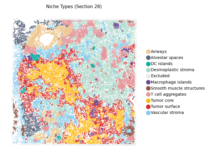
Cell-type spatial map

Load the spatial AnnData and color each cell by its annotated cell type.

color_palette = {
    'Tumor core': "#FDBA12",       
    'Tumor surface': "#D62828",     
    'Desmoplastic stroma': "#ABD8C9",   
    'Smooth muscle structures': "#8d5749",  
    'T cell aggregates': "#E5989B",     
    'Macrophage islands': "#6A4C93",   
    'DC islands': "#08ada4",            
    'Airways': "#EEC994",               
    'Vascular stroma': "#83ccec",       
    'Alveolar spaces': "#5C677D",      
    'Excluded': "#EAEAEA"
}

adata = sc.read_h5ad(f'{file_dir}/NSCLC_section_28.h5ad')
adata.obs['niches_3D'] = adata.obs['niches_3D'].astype('category')

sc.pl.spatial(
    adata,
    color='niches_3D',
    spot_size=4.5,
    palette=[color_palette[c] for c in adata.obs['niches_3D'].cat.categories],
    title='Niche Types (Section 28)',
    legend_loc='right margin',
    show=False,
)
fig = plt.gcf()
plt.show()

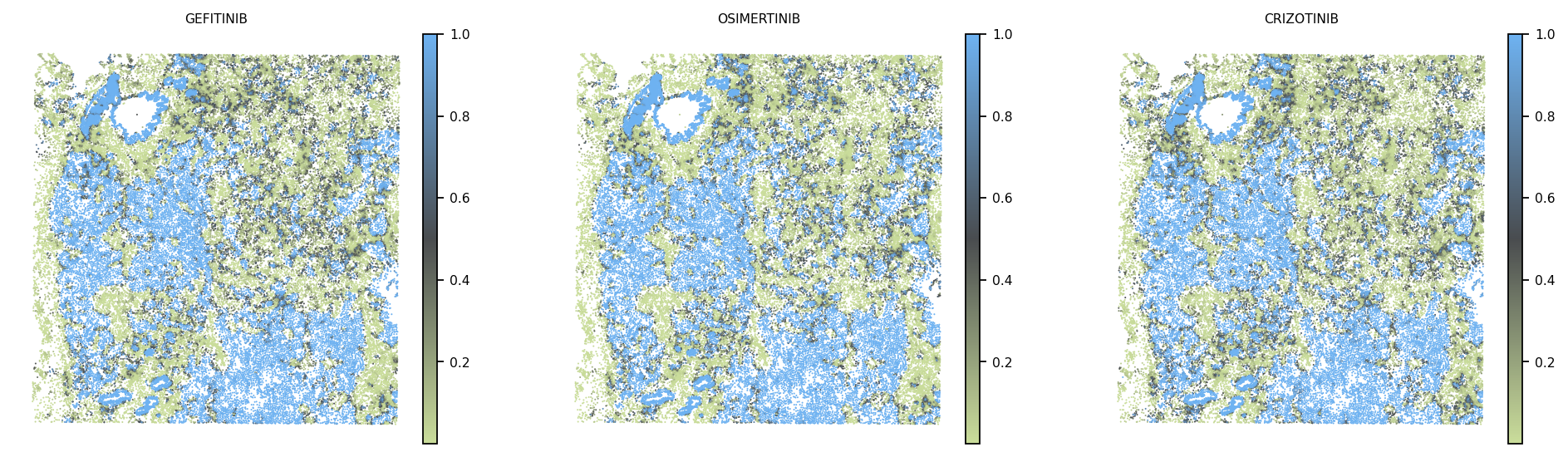
Drug-response spatial maps

pharost.analysis.load_response_prediction populates adata.obs[{drug}] from each drug’s predicted_probabilities.csv. The spatial plot then shows the probability distribution across the tissue.

adata = pharost.analysis.load_response_prediction(
    adata,
    drugs=selected_drugs,
    path_template=lambda d: f'{result_dir}/{d}/predicted_probabilities.csv',
)

drug_cmap = LinearSegmentedColormap.from_list(
    'pink_yellow_teal', ['#CADD9B', '#494C4F', '#6EB2F1'], N=256,
)

sc.pl.spatial(
    adata, color=selected_drugs, spot_size=4.5,
    cmap=drug_cmap, vmax=1, show=False,
)
fig = plt.gcf()

os.makedirs('figures_NSCLC', exist_ok=True)
plt.savefig('figures_NSCLC/01_Spatial_drug_response.png', bbox_inches='tight', dpi=500)
plt.show()

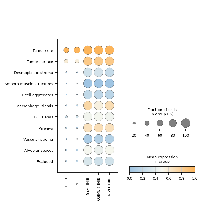
Marker-gene + drug-response dotplot

Compare canonical breast-cancer markers (ERBB2, ESR1, PGR) against predicted drug responses in one dotplot, grouped by cell type.

var_names = ['EGFR', 'MET'] + selected_drugs

dot_cmap = LinearSegmentedColormap.from_list(
    "blue_white_orange", ["#A0C5E3", "#F7F8F0", "#FCB55C"]
)
sc.pl.dotplot(
    adata,
    var_names=var_names,
    groupby='niches_3D',
    categories_order=list(color_palette.keys()),
    standard_scale='var',
    cmap=dot_cmap,
    show=False,
)
plt.savefig('figures_NSCLC/01_Drug_gene_dotplot_summary.png', bbox_inches='tight', dpi=300)
plt.show()

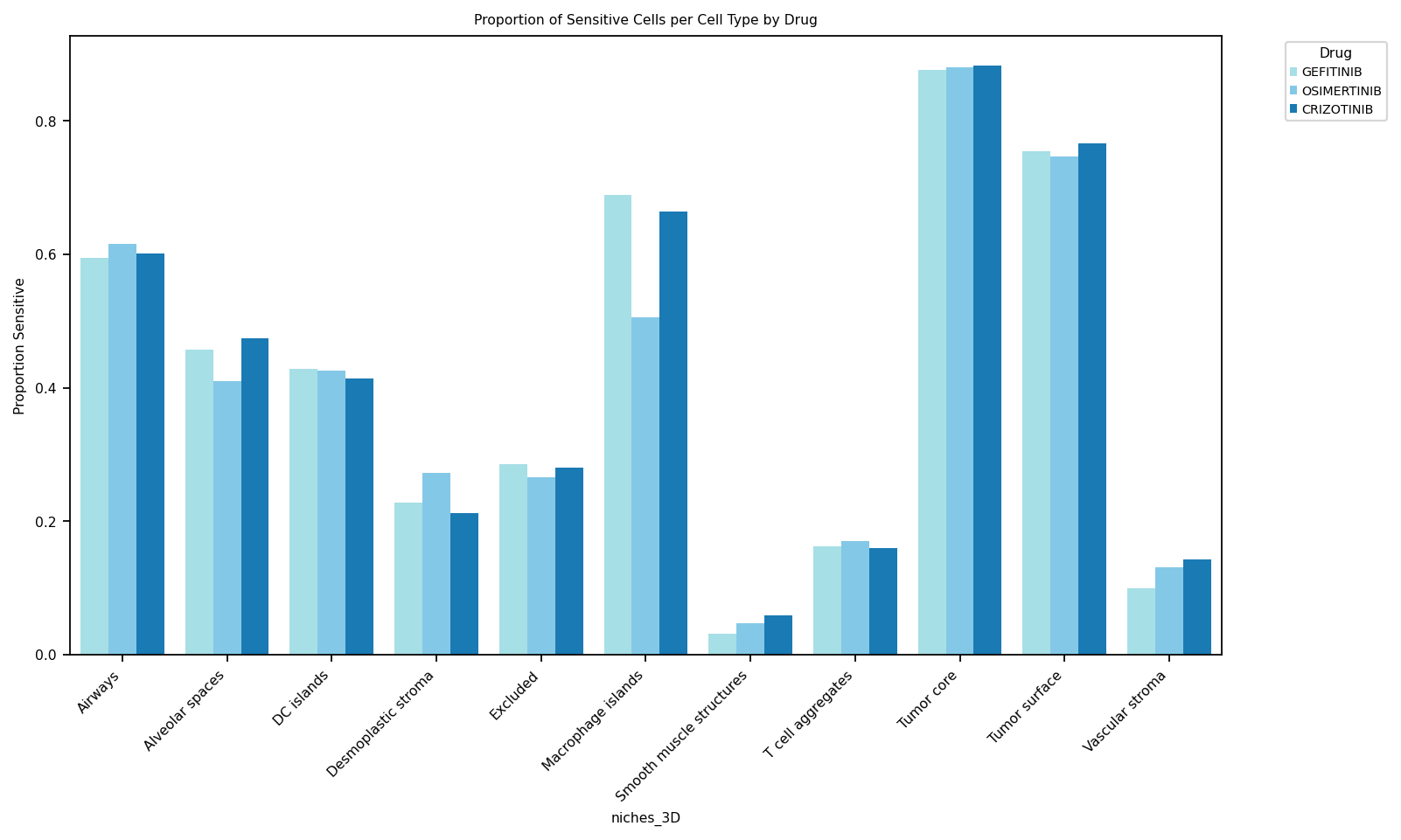
Sensitive-cell proportion per cell type

For each drug, plot the fraction of cells with predicted probability > 0.5 within each cell type. Highlights which populations the model considers sensitive.

pharost.analysis.plot_response_celltype_prop(
    adata,
    target_drugs=selected_drugs,
    cell_type_col='niches_3D',
    save=True,
    file_format='pdf',
    palette = ['#9BE8F0', '#74CEF7', '#0180CC'], 
    save_dir='figures_NSCLC',
)

Figure saved to figures_NSCLC/response_celltype_prop.pdf